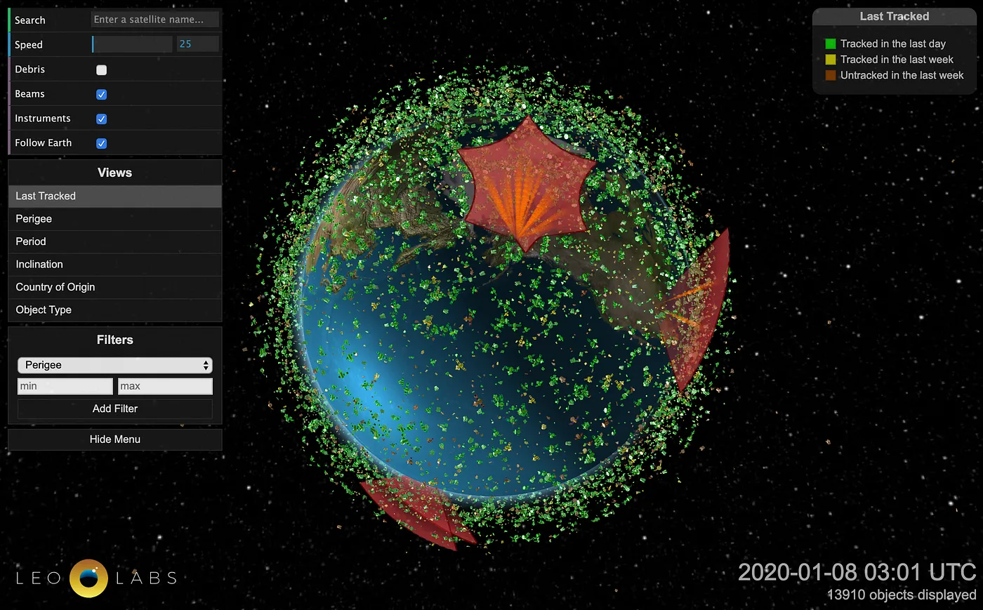
In addition to tracking thousands of objects in Low Earth Orbit (LEO) with our network of phased-array radar systems, LeoLabs also searches for potential conjunction events that can pose a danger to satellite operators. Our system detects and analyzes roughly 800,000 potential collision scenarios each day.
The vast majority of high risk conjunction events are not between active satellites, but rather between inactive objects such as orbital debris, spent rocket bodies, or inactive satellites.
This is not surprising, since only about 10% of the objects currently tracked in LEO are actively working satellites. For this inaugural blog post, let’s take a closer look at how we identify conjunctions and quantify risk for these events.
How Conjunction Risk is Calculated
There are multiple steps required to accurately characterize the risk of a collision occurring between two objects in space. Conjunction Data Messages, or CDMs, have long been the industry standard data product for quantifying risk for these types of events. They provide key information such as the IDs of the two objects that may collide, the time of closest approach (TCA), their positions and velocities, miss distance, Probability of Collision (Pc), and the computed measurement uncertainties for each object at TCA.
To understand CDMs, we first have to explain how Pc is calculated, and for that we need to understand the concept of a state vector and its associated uncertainty. The state vector is the position and velocity of an object at a particular time, known as the epoch. It is determined by fitting physical orbits through a series of recent observational passes, and looking for the orbital state vector which best fits those observations. Every time an object is tracked passing over one of our radars, we incorporate the new measurements and fit for an updated state vector at the new epoch corresponding to the time of the radar pass. There is never perfect knowledge of a state vector due to measurement errors, which means that even at epoch there is some level of uncertainty. This uncertainty arises because there is actually a range of state vectors which are all consistent with the observations. This uncertainty in the state vector will turn out to be a critical quantity in assessing collision risk.
From the orbital state vector, the position of the object can be propagated forward in time from the epoch to form a list of positions versus times in the future. This is known as an ephemeris. As mentioned earlier, there is uncertainty to these positions even at epoch due to measurement errors (LeoLabs measures the range to each target typically with an uncertainty of less than 15 meters). Furthermore, this uncertainty grows with time as it is propagated into the future. To add to this, there is also a component of uncertainty due to variations in the atmospheric drag profile of LEO objects which depends upon things like solar activity and the size, shape, and orientation of the object. Typically, the uncertainty from atmospheric drag comes to dominate after a few days of propagation in LEO, especially as we go lower in altitude. Thus, even if we knew exactly where a space object is at some given time, there would still be uncertainty in calculating its future location. It is critical that as part of the ephemeris we also calculate the growing uncertainties at each time step into the future, because that will form the basis for calculating potential collision probabilities.
Once we have ephemeris files for the objects we are tracking, we can search forward in time to find instances in the next seven days where two objects will be in close proximity. The fact that the fitted state vectors of two objects will pass close to each other does not tell the whole story though, as each of those state vectors has an associated uncertainty which must be taken into account in order to understand the seriousness of the event. Once we have all these pieces in place, we can now move to calculate the Pc using well known algorithms. The Pc is calculated by taking into account the range of possible positions of the two objects and finding what fraction of trajectories actually collide.
A Recent Close Approach
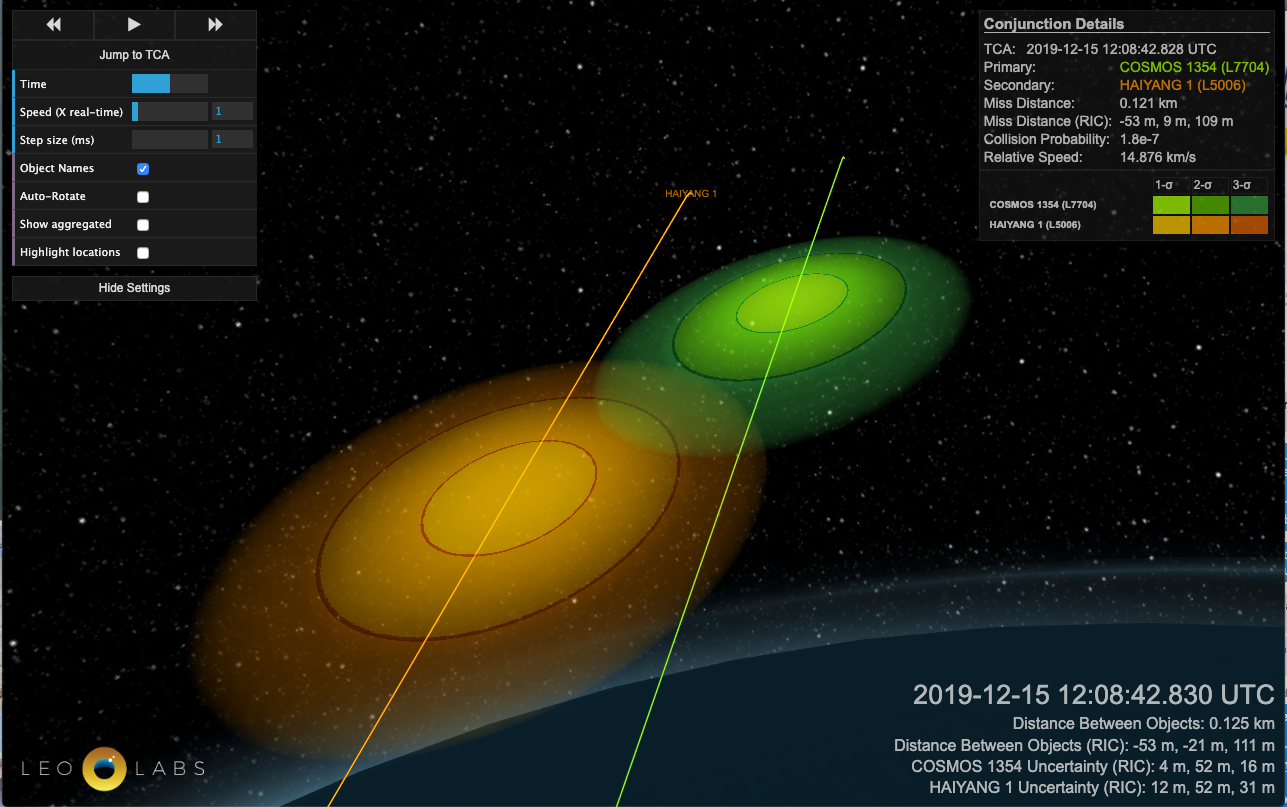
On December 8, 2019, LeoLabs determined that the Haiyang 1 and Cosmos 1354 satellites had an upcoming close approach on December 15 that was of concern. This link shows the evolution of the event over eight days, during which time our system generated 52 CDMs (one for each new state vector update on either object). Click on the map to see the ground track of the two objects and on the “View in 3D” button to visualize the event.
Let’s look at the evolution of computed risk for this event.
- Seven days prior to TCA: Upon initial event detection, a Pc of 1.6e-4 and miss distance of 158 (+/-308) meters
- Five days prior to TCA: Pc has increased to 8.9e-3 and miss distance of 39m (+/-192)
- Three days prior to TCA: Pc has increased again to 1.8e-2 and miss distance of 13m (+/-111)
This turned out to be the highest risk CDM generated over the course of the event. These computed risk values can and often do fluctuate from one CDM update to the next due to reasons described above. Luckily as we got closer to TCA, subsequent updates for this event showed the risk starting to decrease.
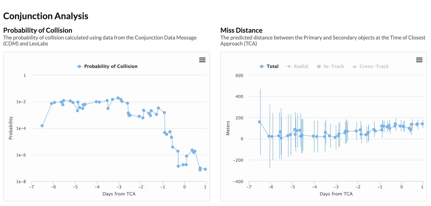
- 2.5 days to TCA: Pc has decreased to 9.7e-4 and miss distance of 69m (+/-80)
- 21 hours to TCA: Pc has decreased to 4.6e-5 and miss distance of 119m (+/-55)
- 1 hour to TCA: Pc has decreased to 1.8e-7 and miss distance of 121m (+/-47)
So why did the collision probability fall so quickly in the last 24 hours? As we approached TCA, the computed miss distance increased slightly, while our uncertainty in the miss distance further decreased. Note that regardless of the reported miss distances above, the (+/-) margin of uncertainty always decreases as we approach TCA. Eventually, our uncertainties in the spacecraft positions fell below the predicted distance of close approach, resulting in our being able to confidently rule out this as a collision roughly 24 hours prior to TCA.
Herein lies an advantage of a distributed global sensor network: frequent radar observations yield more frequent and more accurate state vectors, due to minimized uncertainty growth in between updates. For this conjunction event, our system provided new state vectors more than six times per day on average.
This conjunction risk information is also graphically depicted in the Error Ellipse section where we show the evolution of the relative position prediction. Zoom in and hover over some of the plot ellipsoids to see the values (each one corresponding to a CDM).
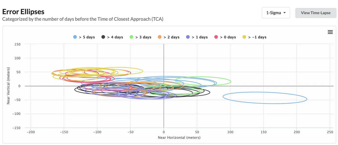
The origin of the plot (0,0) represents the center of mass of the primary object. The location of each ellipsoid represents the distance of the center of mass of the secondary object to the primary object at TCA, and the size of the ellipsoid corresponds to our calculated positional uncertainties for the two objects (smaller ellipsoids mean lower uncertainty, and better confidence in the accuracy of our state vectors).
Keep in mind that the estimate of the Pc depends on the size and orientation of the two objects, which we do not know exactly. In other words, the smaller the two objects, the closer they have to be to (0,0) in order for there to be a collision. In this case, both objects were large spacecraft, and for the purposes of estimating Pc we assume the sum of the linear size of the two spacecraft to be five meters. This is known as the combined hard body radius (HBR), and this assumption is listed at the top of the Conjunction Analysis Report.
Finally, at the bottom of the page we depict how varying the combined HBR and state vector uncertainties will affect the computed Pc value. In some instances, Pc results can be extremely sensitive to small variations in inputs to the algorithm. As we can see in this example, if we keep the same HBR but decrease our uncertainties by 50% (thus, our knowledge of position is improved by 50%), the already low final Pc value of 8.1e-8 drops by another 16 orders of magnitude!
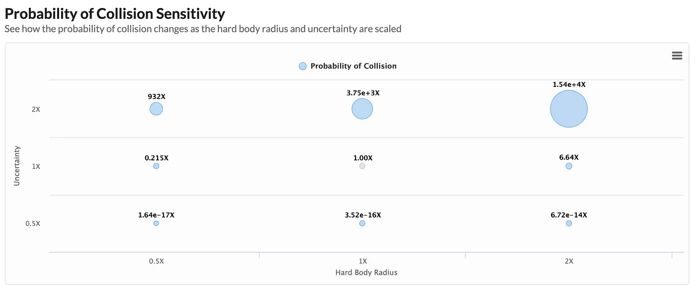
As there is no one “correct” Pc for any conjunction event (in reality, either the objects will hit or they won’t), these sensitivity diagrams are helpful to understand collision risk in the larger context of the assumptions used in computing it. We can also see the value in having a large number of CDMs generated for each event so that we can study the data in aggregate, identifying patterns and trends from one update to the next as we attempt to better understand the event risk.
Final Observations
This example demonstrates the power of the LeoLabs worldwide network of radars. The more frequently objects are tracked, the smaller the uncertainty in the state vectors at epoch (i.e. the more tracking data we have, the better we can fit the state vector) and the more recent the latest epoch time will be. This results in earlier determination either that a potential collision is not of concern, or in cases where the close approach is within the uncertainty region, that a collision is possible and a collision avoidance maneuver is warranted. LeoLabs currently has three operational radars, and plans to build three more over the next two years to further improve our space tracking services. Our completed radar network will be capable of monitoring a predicted catalog of 250,000 objects including small debris down to 2cm in size, while continuously monitoring for dangerous conjunctions.
These capabilities described will become available to satellite operators worldwide as a commercial collision prevention service starting in Spring 2020.